此次笔记是对前两周学习内容的查漏补缺
一些基本函数
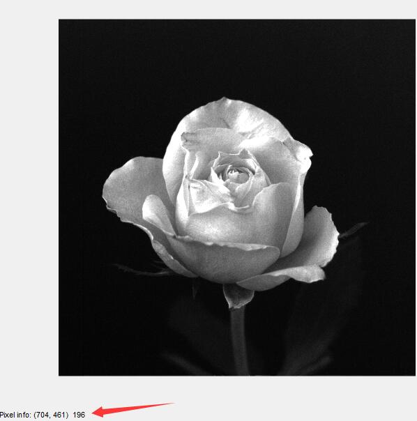
函数impixelinfo
图像的转换
| function | use | format |
| ——– | ——————– | ———————- |
| ind2gray | indexed to grescale | y = ind2gray(x, map) |
| gray2ind | grayscale to indexde | [y, map] = gray2ind(x) |
| rgb2gray | RGB to grayscale | y = rgb2gray(x) |
| gray2rgb | grayscale to RGB | y = gray2rgb(x) |
| rgb2ind | RGB to indexed | [y, map] = rgb2ind |
| ind2rgb | indexed to RGB | y = ind2rgb(x, map) |im2double 和double 的区别
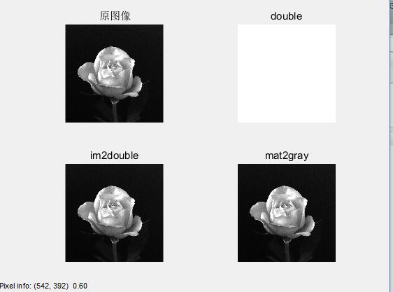
double 就是见到地把有个变量的类型转换成double 型,数值大小不变
im2double 函数,如果输出的是uint8 uint16 或logical 类型,则函数im2double 将其值归一到0 ~1 之间
如果输入本身就是double 类型,则输出还是double型,并不进行归一化
mat2gray是将图像矩阵归一化操作,常用的为A = im2uint8(mat2gray(image)) 这样就将矩阵转化为uint8类型的图像
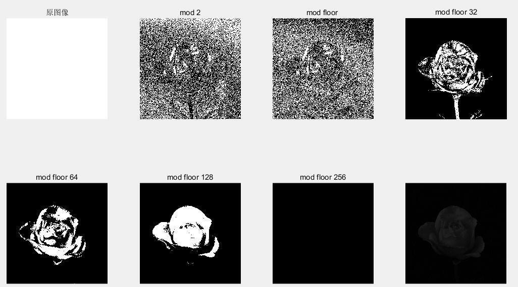
函数mod
除数取余
floor 向下取余
image、函数imagesc 和imshow的区别
三个都可以将 m n 3 的矩阵当做RGB图像来显示,但是imshow 是按照图片原本的尺寸显示,但是imagesc和imshow则是以一定的比例缩放后显示
显示灰度图像
我们需要明确什么是索引图像
当Matlab中的imread函数将图像读入并存入矩阵时,我们知道如果是RGB图像,得到的是M N 3的矩阵,但如果是索引图像,得到的就是m* n 的矩阵,这个矩阵的每个元素每个元素只是一个数值
如果想通过RGB值来显示一个图像,就要用到colormap
colormap 上节课说过,就是一个m 3 的矩阵,每个矩阵有3列元素构成RGB组,也就是一种颜色,一个m 3 的colormap中有m 种颜色
而索引图像存储的数值和colormap 中的行号对应起来就可以向RGB那样显示图片
image
用image系列绘图的坐标和普通绘图命令得到的坐标在纵轴方向是相反的,可以用axis命令手动设置坐标格式。
axis xy就是普通的坐标格式。
axis ij就是image系列的坐标格式。imagesc
缩放数据并显示图像对象。
使用方法编辑本段回目录 imagesc函数放大图像数据以覆盖当前色图的整个范围,并显示图片。imagesc(C)
将输入变量C显示为图像。C中的每一个元素对应着图像中的一个矩形局域。C中的元素值的对应与色图中的索引,色图决定了每一个补片的颜色。
imagesc(x,y,C)
将输入变量C显示为图像,并且使用x和y变量确定x轴和y轴的边界。如果x(1) > x(2) 或 y(1) > y(2),图像是左右或上下反转的。
imagesc(…,clims)
归一化C的值在clims所确定的范围内,并将C显示为图片。clims是两元素的向量,用来限定C中的数据的范围,这些值映射到当前色图的整个范围。
h = imagesc(…)
返回图像对象的句柄。
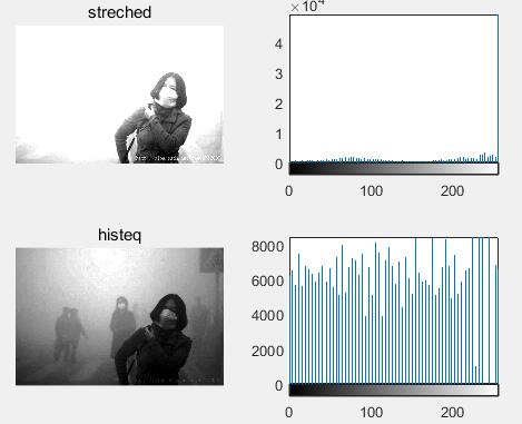
图片增强
1234567>> imh = imadjust(f,[0.3,0.6],[0.0,1.0]);>> imh1 = histeq(f);>> figure;>> subplot(2,2,1);imshow(imh);title('streched');>> subplot(222);imhist(imh);>> subplot(2,2,3);imshow(imh1);title('histeq');>> subplot(224);imhist(imh1);
filter2和imfilter的区别
imfilter可进行多维图像的进行空间滤波,可选参数较多
filter2只能对二维图像进行空间滤波
两个函数结果类型不一样,只需要在I1=filter2(h,I)后面加上I1=uint8(I1)进行类型转换,结果就是一样的。
函数filter2
12Y = filter2(B,X)或 Y = filter2(B, X, 'shape')filter2中使用矩阵B中的二维FIR滤波器对数据X进行滤波,结果Y是通过二维互相关计算出来的,其大小由参数’shape’决定,如果没有该参数值则与X的大小一致
| ‘
full‘ | Returns the full two-dimensional correlation. In this case,Yis larger thanX. |
| ——— | —————————————- |
| ‘same‘ | (default) Returns the central part of the correlation. In this case,Yis the same size asX. |
| ‘valid‘ | Returns only those parts of the correlation that are computed without zero-padded edges. In this case,Yis smaller thanX. |same 与默认的结果相同
123h = ones(3,3)/9;f1 = filter2(h,f,'same');imshow(f1/255);
colormap
在matlab中用来设定和获取当前色图的函数
在matlab中,每一个figure都有一个colormap ,也就是色图
map实际上是一个mx3的矩阵,每一行的3个值都为0-1之间数,分别代表颜色组成的rgb值
例如 : [1 0 0]代表红色 [0 1 0 ]代表绿色 [0 0 1] 代表蓝色
系统中自带一些colormap,也可以定义自己的colormap
colormap只对索引图像有效
控制曲面图的颜色
自定义colormap的颜色
123>> load flujet>> image(X)>> colormap(jet)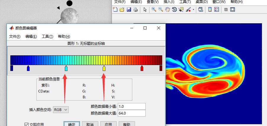
在命令窗口输入 newname = colormap即可对刚才的修改进行保存
之后再调用该colorbar给图片上色的时候直接使用
colormap(newname);
colormap 的色图类型
1234567891011121314151617autumn 从红色平滑变化到橙色,然后到黄色。bone 具有较高的蓝色成分的灰度色图。该色图用于对灰度图添加电子的视图。colorcube 尽可能多地包含在RGB颜色空间中的正常空间的颜色,试图提供更多级别的灰色、纯红色、纯绿色和纯蓝色。cool 包含青绿色和品红色的阴影色。从青绿色平滑变化到品红色。copper 从黑色平滑过渡到亮铜色。flag 包含红、白、绿和黑色。gray 返回线性灰度色图。hot 从黑平滑过度到红、橙色和黄色的背景色,然后到白色。hsv 从红,变化到黄、绿、青绿、品红,返回到红。jet 从蓝到红,中间经过青绿、黄和橙色。它是hsv色图的一个变异。line 产生由坐标轴的ColorOrder属性产生的颜色以及灰的背景色的色图。pink 柔和的桃红色,它提供了灰度图的深褐色调着色。prism 重复这六种颜色:红、橙、黄、绿、蓝和紫色。spring 包含品红和黄的阴影颜色。summer 包含绿和黄的阴影颜色。white 全白的单色色图。winter 包含蓝和绿的阴影色。colormap 每次设定都会改变,使用freezecolors后每次设定的colormap都会保留下来。
函数freezecolors
12345678910>> subplot(2,1,1);>> imagesc(peaks)>> colormap hot>> freezeColors>> cbfreeze(colorbar);>> subplot(2,1,2)>> colormap hsv>> surf(peaks)>> freezeColors>>cbfreeze(colorbar) 1234567891011121314>> f = imread('Fig0602(b)(RGB_color_cube).tif');>> f = rgb2gray(f);>> subplot(2,3,1),imshow(f),title('原图像');>> freezeColors;>> subplot(2,3,2),imshow(f),colormap pink,title('colormap pink');>> freezeColors;>> subplot(2,3,3),imshow(f),colormap copper,title('colormap copper');>> freezeColors;>> subplot(2,3,4),imshow(f),colormap jet,title('colormap jet');>> freezeColors;>> subplot(2,3,5),imshow(f),colormap hot,title('colormap hot');>> freezeColors;>> subplot(2,3,6),imshow(f),colormap colorcube,title('colormap colorcube');>> freezeColors;
函数imagesc
imagesc(A) 将矩阵A中的元素数值按大小转化为不同颜色,并在坐标轴对应位置处以这种颜色染色
imagesc(x,y,A) x,y决定坐标范围,x,y应是两个二维向量,即x=[x1 x2],y=[y1 y2],matlab会在[x1,x2][y1,,y2]的范围内染色。 如果x或y超过两维,则坐标范围为[x(1),x(end)][y(1),y(end)]函数retinex
图像增强算法
基本思想
S(x, y) = R(x, y ) * L(x, y )
其中R代表入射光,L代表反射性之,相当于背景原本应该有的颜色,S代表反射光,也就是获得的图像
log(S(x, y )) = log(R(x, y)) + log(L(x, y))
基本思路就是获得S,估算出R得出物体本身的颜色L
R是低频信号,L是高频信号
对L进行低频滤波得到R,然后对数域下S减去R,就是L了
常用的三个模型
SSR,MSR,MSRCR
SSR是单尺度Retinex
用高斯模板和图像卷积,给图像滤波,得到滤波后的图像
将图像和滤波后的图像都log一下,转到对数域相减
做Exp指数运算,恢复到正常的图像来
MSR是多尺度的
几个不同的参数的搞死模板,不同参数导致锐化程度不同,每个模板都相当于做SSR,得到的几个结果加权相加,一般都去权重相同。
MSRCR是带彩色回复的多尺度Retinex
尽量满足修复后的图像R,G,B三个像素值趋于1:1:1
代码中的算法部分参照网上
123456789101112131415161718192021222324252627282930313233343536373839404142434445464748495051525354555657585960616263646566676869707172737475767778798081828384858687888990919293949596979899100101102103104105106107108109110111112113114115116117118119120121122123124125126127128129130131132133134135136137138139140141142143144145146147148149150151152153154155156157158159160161162163164165166167168169170171172173174175176177178179180181182function retinex(I)Ir=I(:,:,1);Ig=I(:,:,2);Ib=I(:,:,3);%%%%%%%%%%设定所需参数%%%%%%G = 192;b = -30;alpha = 125;beta = 46;Ir_double=double(Ir);Ig_double=double(Ig);Ib_double=double(Ib);%%%%%%%%%%设定高斯参数%%%%%%sigma_1=15; %三个高斯核sigma_2=80;sigma_3=250;[x y]=meshgrid((-(size(Ir,2)-1)/2):(size(Ir,2)/2),(-(size(Ir,1)-1)/2):(size(Ir,1)/2));gauss_1=exp(-(x.^2+y.^2)/(2*sigma_1*sigma_1)); %计算高斯函数Gauss_1=gauss_1/sum(gauss_1(:)); %归一化处理gauss_2=exp(-(x.^2+y.^2)/(2*sigma_2*sigma_2));Gauss_2=gauss_2/sum(gauss_2(:));gauss_3=exp(-(x.^2+y.^2)/(2*sigma_3*sigma_3));Gauss_3=gauss_3/sum(gauss_3(:));%%%%%%%%%%对R分量操作%%%%%%%% MSR部分Ir_log=log(Ir_double+1); %将图像转换到对数域f_Ir=fft2(Ir_double); %对图像进行傅立叶变换,转换到频域中%sigam=15的处理结果fgauss=fft2(Gauss_1,size(Ir,1),size(Ir,2));fgauss=fftshift(fgauss); %将频域中心移到零点Rr=ifft2(fgauss.*f_Ir); %做卷积后变换回空域中min1=min(min(Rr));Rr_log= log(Rr - min1+1);Rr1=Ir_log-Rr_log;%sigam=80fgauss=fft2(Gauss_2,size(Ir,1),size(Ir,2));fgauss=fftshift(fgauss);Rr= ifft2(fgauss.*f_Ir);min1=min(min(Rr));Rr_log= log(Rr - min1+1);Rr2=Ir_log-Rr_log;%sigam=250fgauss=fft2(Gauss_3,size(Ir,1),size(Ir,2));fgauss=fftshift(fgauss);Rr= ifft2(fgauss.*f_Ir);min1=min(min(Rr));Rr_log= log(Rr - min1+1);Rr3=Ir_log-Rr_log;Rr=0.33*Rr1+0.34*Rr2+0.33*Rr3; %加权求和MSR1 = Rr;SSR1 = Rr2;%计算CRCRr = beta*(log(alpha*Ir_double+1)-log(Ir_double+Ig_double+Ib_double+1));%SSR:min1 = min(min(SSR1));max1 = max(max(SSR1));SSR1 = uint8(255*(SSR1-min1)/(max1-min1));%MSRmin1 = min(min(MSR1));max1 = max(max(MSR1));MSR1 = uint8(255*(MSR1-min1)/(max1-min1));%MSRCRRr = G*(CRr.*Rr+b);min1 = min(min(Rr));max1 = max(max(Rr));Rr_final = uint8(255*(Rr-min1)/(max1-min1));%%%%%%%%%%对g分量操作%%%%%%%Ig_double=double(Ig);Ig_log=log(Ig_double+1); %将图像转换到对数域f_Ig=fft2(Ig_double); %对图像进行傅立叶变换,转换到频域中fgauss=fft2(Gauss_1,size(Ig,1),size(Ig,2));fgauss=fftshift(fgauss); %将频域中心移到零点Rg= ifft2(fgauss.*f_Ig); %做卷积后变换回空域中min2=min(min(Rg));Rg_log= log(Rg-min2+1);Rg1=Ig_log-Rg_log; %sigam=15的处理结果fgauss=fft2(Gauss_2,size(Ig,1),size(Ig,2));fgauss=fftshift(fgauss);Rg= ifft2(fgauss.*f_Ig);min2=min(min(Rg));Rg_log= log(Rg-min2+1);Rg2=Ig_log-Rg_log; %sigam=80fgauss=fft2(Gauss_3,size(Ig,1),size(Ig,2));fgauss=fftshift(fgauss);Rg= ifft2(fgauss.*f_Ig);min2=min(min(Rg));Rg_log= log(Rg-min2+1);Rg3=Ig_log-Rg_log; %sigam=250Rg=0.33*Rg1+0.34*Rg2+0.33*Rg3; %加权求和SSR2 = Rg2;MSR2 = Rg;%计算CRCRg = beta*(log(alpha*Ig_double+1)-log(Ir_double+Ig_double+Ib_double+1));%SSR:min2 = min(min(SSR2));max2 = max(max(SSR2));SSR2 = uint8(255*(SSR2-min2)/(max2-min2));%MSRmin2 = min(min(MSR2));max2 = max(max(MSR2));MSR2 = uint8(255*(MSR2-min2)/(max2-min2));%MSRCRRg = G*(CRg.*Rg+b);min2 = min(min(Rg));max2 = max(max(Rg));Rg_final = uint8(255*(Rg-min2)/(max2-min2));%%%%%%%%%%对B分量操作同R分量%%%%%%%Ib_double=double(Ib);Ib_log=log(Ib_double+1);f_Ib=fft2(Ib_double);fgauss=fft2(Gauss_1,size(Ib,1),size(Ib,2));fgauss=fftshift(fgauss);Rb= ifft2(fgauss.*f_Ib);min3=min(min(Rb));Rb_log= log(Rb-min3+1);Rb1=Ib_log-Rb_log;fgauss=fft2(Gauss_2,size(Ib,1),size(Ib,2));fgauss=fftshift(fgauss);Rb= ifft2(fgauss.*f_Ib);min3=min(min(Rb));Rb_log= log(Rb-min3+1);Rb2=Ib_log-Rb_log;fgauss=fft2(Gauss_3,size(Ib,1),size(Ib,2));fgauss=fftshift(fgauss);Rb= ifft2(fgauss.*f_Ib);min3=min(min(Rb));Rb_log= log(Rb-min3+1);Rb3=Ib_log-Rb_log;Rb=0.33*Rb1+0.34*Rb2+0.33*Rb3;%计算CRCRb = beta*(log(alpha*Ib_double+1)-log(Ir_double+Ig_double+Ib_double+1));SSR3 = Rb2;MSR3 = Rb;%SSR:min3 = min(min(SSR3));max3 = max(max(SSR3));SSR3 = uint8(255*(SSR3-min3)/(max3-min3));%MSRmin3 = min(min(MSR3));max3 = max(max(MSR3));MSR3 = uint8(255*(MSR3-min3)/(max3-min3));%MSRCRRb = G*(CRb.*Rb+b);min3 = min(min(Rb));max3 = max(max(Rb));Rb_final = uint8(255*(Rb-min3)/(max3-min3));%%%%%%%%%%%%%%%%%%%%%%%%%%%%%%%%%%%%%%%%%ssr = cat(3,SSR1,SSR2,SSR3);msr = cat(3,MSR1,MSR2,MSR3);msrcr=cat(3,Rr_final,Rg_final,Rb_final); %将三通道图像合并subplot(2,2,1);imshow(I);title('原图') %显示原始图像subplot(2,2,2);imshow(ssr);title('SSR')subplot(2,2,3);imshow(msr);title('MSR')subplot(2,2,4);imshow(msrcr);title('MSRCR') %显示处理后的图像
双边滤波
双边滤波是一种可以保边去噪的滤波器。
双边滤波器的实现
函数bfilter2
1function B = bfilter2(A,w,sigma)其中 A 为输入图像,归一化到[0, 1]的矩阵
w 为双边滤波器 的边长\2
定义域方差记为sigma(1) , 值域方差为sigma(2)
123456>> f = imread('iris.tif');>> w = 5;>> f = double(f)/255;>> sigma = [3 0.1];>> h = bfilter2(f, w, sigma);>> imshow(h);